Using Shuffle for Data Anonymization

Data anonymization is a popular topic today for both enterprise and open public data uses.  Less commonly used techniques are data shuffling and swapping, techniques which work well when retention of data distribution is important.  For example, retaining the age distributions of employees.

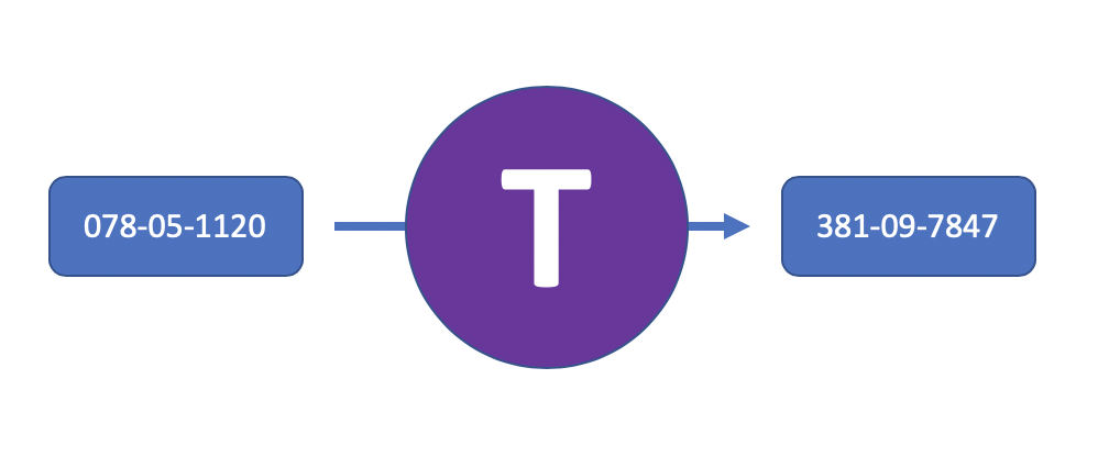
Shuffling data reorders one or more columns so that the statistical distribution remains the same but the shuffled values no longer can be used to re-identify entities in rows.  Since shuffling doesn’t remove or alter uniquely identifying individual values, it may need to be combined with other techniques to properly anonymize a data set. 

Random Shuffle

Basic data shuffling will randomly permute a list of elements.  Consider as an example, an open public data set for the City of Atlanta employee salary data in 2015.  This data is in the public record, and contains the employees' full names, ages and salaries. 

We'll start de-identification by first replacing each employee’s name with a sequential ID.  

Original public data with name replaced:

Employee	Age	Annual Salary
0001	38	46,000
0002	52	26,700
0003	44	46,575
0004	42	42,867
0005	32	28,035
0006	44	67,800
0007	33	46,378
0008	28	39,328
0009	58	125,000
0010	45	60,466

To further de-identify the data set, while preserving data utility, we might shuffle the age column. Quasi-identifiers are attributes which do not uniquely identify an individual, but are sufficiently correlated that they can sometimes or when combined with other data can be used to re-identify someone. 

Shuffling the age column removes the correlation between age and salary.  The statistical distributions of age and salary are unaffected with this approach.

With age shuffled:

Employee	Age	Annual Salary
0001	44	46,000
0002	28	26,700
0003	44	46,575
0004	38	42,867
0005	52	28,035
0006	45	67,800
0007	42	46,378
0008	32	39,328
0009	58	125,000
0010	33	60,466

Shuffling Data

All permutations are equally likely when shuffling, including the original list.  In this instance, run using python's shuffle, employee 0003's age after shuffling retained the same value.

Data shuffling has been endorsed by the EU Data Protection Board in 2014 which wrote:

Shuffling the values of attributes in a table so that some of them are artificially linked to different data subjects, is useful when it is important to retain the exact distribution of each attribute within the dataset

Similarly to noise addition, permutation may not provide anonymisation by itself and should always be combined with the removal of obvious attributes/quasi-identifiers.

Many ETL tools provide shuffling as a de-identification technique, including Talend, Informatica, Ab Initio and even Oracle.  

History of the Fisher-Yates Shuffle

The first shuffle algorithm was described by Ronald Fisher and Frank Yates in their 1938 book Statistical tables for biological, agricultural and medical research.  A software version of the algorithm, optimized by Richard Durstenfeld to run in linear O(n) time, was popularized in Donald Knuth’s The Art of Computer Programming Volume II.  

Below is a python example of this algorithm:

import random 

list = [38, 52, 44, 42, 32, 44, 33, 28, 58, 45]

print ("The original list is : " + str(list)) 

# Fisher–Yates Shuffle

for i in range(len(list)-1, 0, -1): 

    # Pick a random index from 0 to i  

    j = random.randint(0, i + 1)  

    

    # Swap arr[i] with the element at random index  

    list[i], list[j] = list[j], list[i]  

      

print ("The shuffled list is : " +  str(list))

Python and Java, however, provide built-in shuffle methods.  Below is python code to shuffle the employee ages in the example above: 

list = [38, 52, 44, 42, 32, 44, 33, 28, 58, 45]

random.shuffle(list)

[44, 28, 44, 38, 52, 45, 42, 32, 58, 33]

Well Known Uses

The U.S. Census Bureau began using a variant of data swapping for the 1990 decennial census. The method was tested with extensive simulations, and the results were considered to be a success and essentially the same methodology was used for actual data releases.  In the U.S. Census Bureau’s version, records were swapped between census blocks for individuals or households that have been matched on a predetermined set of k variables.  A similar approach was used  for the U.S. 2000  census. The Office for National Statistics in the UK applied data swapping as part of its disclosure control procedures for the U.K. 2001 Census.

In 2002, researchers at the U.S. National Institute of Statistical Science (NISS) developed WebSwap, a public web-based tool to perform data swapping in databases of categorical variables.

Other Shuffle and Swapping Techniques

Group shuffle is used when two or more rows need to be shuffled together.  Some data sets may have columns with highly correlated data, so shuffling a single column in isolation would diminish the analytical value of the data.  

Consider our earlier employee example with the addition of a years-of-service column.  Since a persons age is related to their potential employment longevity, it would make sense to shuffle these together.

Direct swapping is a non-random approach which handpicks records by finding pairs to swap.  For a record set with age and salary, you can swap the salary of individuals of the same age. For example the following rows :

Dept. Id	Age	Annual Salary
A03031	44	95,000
A68002	44	60,000

swapping salary where age = 44:

Dept. Id	Age	Annual Salary
A03031	44	60,000
A68002	44	95,000

Direct swapping works with categorical data (e.g., eye color green, blue, brown or black) or a discrete number of values, in our example age represents a range 0..110.

   

Rank swap is similar, swapping pairs which are not exact matches, but close in value. It works well on continuous variables. For example blood pressure within 5 hg could be chosen as  pairs to swap:

original:

Systolic Blood Pressure (Hg)	Height	Weight
121	5' 8"	155
122	5' 11"	180

swapped:

Systolic Blood Pressure (Hg)	Height	Weight
121	5' 11"	180
122	5' 8"	155

In practice, both direct and rank swapping typically swap a subset of the records, not the entire set.

  

Summary

Shuffle can be applied as one of several valuable techniques for data de-identification.  As the EU Data Protection Board recommends, it may not be appropriate for stand-alone use, and always requires careful analysis with a given data set that obvious identifiers and quasi-identifiers are protected.  Consider applying a k-anonymization test on the output data.

How Tokenized Data Protected Capital One When Encryption Failed

The Capital One data breach this past August impacted over 100M individuals but provided some important lessons and a few silver linings. With so many affected, the FBI’s quick arrest of the perpetrator was met with relief and questions of what had happened to the data. Although the data had been downloaded and posted privately on Github, the actual data was never sold or disseminated. In fact, much of the highly sensitive data, in particular Social Security and account numbers, had been "tokenized" and therefore remained secure.

Roughly 99% of the Social Security Numbers were protected. But why then were some 140,000 SSNs exposed? As it turns out, those that were exposed had not been tokenized. As per Capital One’s policies, all American SSNs should be and were tokenized. But, Capital One's policies did not require tokenizing the employee ID field, which in some cases consisted of a SSN. Also, the equally sensitive Canadian Insurance Numbers, with a slightly different format than the US numbers, were not tokenized and over 1M were exposed.

Data privacy professionals should note the importance of tokenizing data over encryption. The attacker in this instance gained unauthorized access to the encryption keys, and the encrypted data was then successfully decrypted and breached. Tokenized data, however, remained fully protected.

As illustrated by this incident, the risk of theft or misuse of an encryption key remains a major hurdle to fully securing data with encryption. The bank exposed the most sensitive PII (Personally Identifiable Information) tied to some of its US and Canadian customers when encryption failed to protect the data.

Tokenization

Tokenization methods vary, but the process is simple: a data field with a sensitive, personal identifier is replaced with a different, synthetic value, of the same format. Tokenization is usually performed consistently, whereby each unique value is always converted to another unique value within a data set. It is consistent, so the translation from original to synthetic value is the same, every time. Thus, a relational database using SSN as a key can still join on the synthetic SSN.

Payment vendor Square reports that ‘payment experts are seeing more and more organizations moving from encryption to tokenization as a more cost-effective (and secure) way to protect and safeguard sensitive information.“

The most frequenlty stolen Social Security Number of all time is 078-05-1120. The story behind the stolen SSN dates back to 1938 when Douglas Patterson, VP of E.H. Ferree Company, used his secretary’s real SSN on thousands of example Social Security Cards. The purpose of the fake card with a real number was to demonstrate how well it fit into a new line of wallets. Although the sample card was labeled specimen and printed in red instead of blue, the SSN was eventually used by over 40,000 people, some of whom had thought that the card in their wallet was their own.

SSN 078-05-1120 is now a retired number; so let’s use it as an example. The tokenization process would transform this into a synthetic number of exactly the same format, but no longer represents the original value: 

Tokenization can have another benefit. When the format is preserved, and the values are constrained (e.g., digits), the output can be indistinguishable from a real value. In the case of Capital One, it’s unlikely the hacker knew that the SSN values were synthetic, and not real values. According to the FBI, she wrote:

Unknown to the hacker, the SSNs were tokenized, so they were synthetic values unrelated to real Social Security Numbers.  Had Capital One also tokenized Canadian Insurance Numbers and employee ID fields, its likely none of these numbers would have been breached

Random Tokenization

Capital One appears to have used a tokenization technique, known as Format Preserving Encryption (FPE), which itself uses encryption. Had these keys, used by FPE, also been stolen, the tokenized data could have been decrypted.

A better approach is random tokenization, whereby, as the term implies, the tokens are selected randomly. Random tokenization uses a separate key-value database or token vault to consistently tokenize the input data. Unlike encryption, random tokenization does not rely on a single set of keys and the tokens are not vulnerable to mathematical or brute force attacks.

As Jonathan Deveaux wrote in Payments Journal: tokenization "can address the failings of encryption” and “if a hacker was successful and gained access to the tokenized data, it would still be protected as the information would have no exploitable value.”

Summary

Tokenization is recognized as a highly effective data protection technique, and the Capital One incident clearly illustrates its value and effectiveness.

Capital One had policies for tokenizing SSN data. Had Capital One simply tokenized more fields with PII data, neither the SSN or CIN numbers would have been breached and their financial exposure, estimated at $100-$150M, would likely be limited. In contrast, encryption as a data protection policy, remains highly vulnerable to theft or mis-use of the necessary encryption keys. 

References

Payment Tokenization Explained

Why Tokenization Is Key When It Comes to Security and Compliance for the Modern PSP, Payments Journal, July 25, 2019

Capital One Hack Explained: What’s in your Bucket?, Peerlyst, July 30, 2019

United States of America vs Paige A Thompson a/k/a “erratic”, US District Court for the Western District of Washington, July 29, 2019